|
Tutorial
Configuration
Environment managment
Graph managment
Rules managment
Execution managment
|
Graph Managment
The graph is the central concept of GPaR. It is a pregraph such that
- a port is connected to at most one node,
- a port is connected to at most one port.
In this context, encoding classical graph edges between nodes necessitates the use of 2 ports and 3 edges. We will call a classical graph edge a link .
A link between two nodes n1 and n2 is encoded as two port-node edges (p1,n1) and (p2,n2) with p1 and p2 being ports which are linked via the port-port edge (p1,p2).
Moreover, nodes, ports and edges can have attributes. By default, nodes have there 3D-positions as attributes. Additional attributes on nodes, on ports and also on edges have to be defined in the state window.
Initial graph construction
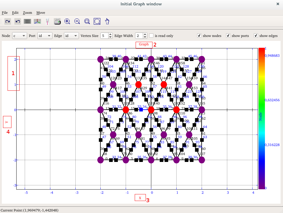
To define the initial graph, click on the  . The initial graph window appears: . The initial graph window appears:
<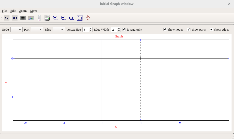 |
Graph window |
By default, it is impossible to modify the graph since the drawing area is in read only mode:
 |
graph window tools bar |
To insert new vertices and edges in the drawing area, this option should be unchecked.
Right click somewhere inside the editor to make the popup menu 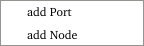 appear.
Select the type of vertex you want to create. The position of this new vertex is the position of your pointer's mouse.
To move the vertex, put the mouse on it and just move it. appear.
Select the type of vertex you want to create. The position of this new vertex is the position of your pointer's mouse.
To move the vertex, put the mouse on it and just move it.
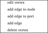
To create an edge between two vertices, right click on the source vertex to make appear the vertex popup menu:
 |
vertex popup menu |
- add edge will add an edge between source vertex and the existing target vertex which is at the pointer of the mouse.
- add edge to node will add an edge between the source vertex and the new node created at the pointer of the mouse if it does not exist.
- add edge to port will add an edge between the source vertex and the new port created at the pointer of the mouse if it does not exist.
- delete vertex will delete the source vertex.
- edit vertex will edit the state of the vertex, the state then can be modified. (see the vertex state settings section )
A shortcut function is included in add edge and add edge to node , it allows to create in one click a link between 2 nodes. This function will create an edge node-port, a port, an edge port-port, a port an edge port-node, and optionally the target node.
Moreover, during the construction of the initial graph, the graph conditions must be satisfied.
It is not allowed to construct, from a given port, 2 port-port connections. In the same way, it is not allowed to construct, from a given port, 2 port-node connections. In both cases, the second edge is not created and an error message appears.
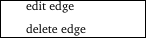
To delete or edit the state of an edge, put the mouse's pointer on the edge and
click on the right button of the mouse. The edge popup menu appears and the desired action can be apply by clicking on one item.
 |
edge popup menu |
To clear all the graph, select the menu Edit->clear graph from the initial graph window menu bar.
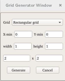
In GPaR a grid generator have been added in the menu Edit->generate grid of the initial graph window menu bar.
 |
Generate grid options |
To generate a mesh in the rectangle [Xmin,Xmax] × [Ymin,Ymax], fill in the boxes xmin, Ymin,
width=Xmin -Xmax and height=Ymin -Ymax. The last boxes you have to fill in correspond to the refinement of the rectangle. More precisely, let us denote nRows and nCols these two integers, (nRows+1)(nCols+1) nodes are created and there coordinates are (Xmin+ × i, Ymin+ × j ) for all integer i between 0 and nRows and for all integer j between 0 and nCols. In addition, ports, edges and also nodes are added depending on the type of the mesh you have selected.
Four different type of meshes are available :
- Rectilinear grid: The set of nodes of this graph is named N and is composed of the (nRows+1)(nCols+1) nodes previously defined. Moreover two nodes of N with coordinates (x,y) and (x',y') are linked if x=x' ± xor y=y' ±.
Thus, the graph contains 2(nRows+1)(nCols+1) ports and 3(nRows+1)(nCols+1) edges. Finally, it is a planar graph containing nRows × nCols cells. When width=height, the grid is a cartesian grid and it can be viewed as the mesh of a 2 dimensional cellular automaton with a Von Neumann neighborhood.
-
Right-angle triangular mesh : it corresponds to the rectilinear grid where the rectangles are cut in half along the diagonal. The set of nodes is again N. Two nodes of coordinates (x,y) and (x',y') are linked if (x=x' ± xor y=y' ±) or (x=x' + and y=y' + ) or (x=x' - and y=y' -). Inside the mesh, all the nodes which not belong to a border have degree 6 . It is a grid formed by tiling the plane regularly with right-angled triangles.
-
Isosceles triangular mesh : The rectilinear grid is expand by a set N' of nRows ×nCols new nodes. there coordinates are: (xmin+ + × i, Ymin++ × j ) for all integer i between 0 and nRows-1 and for all integer j between 0 and nCols-1.
In addition, the nodes of N' are linked to the 4 closest nodes of N.
The degree of nodes belonging to N' is 4. The degrees of nodes of N are 8, 3,4 or 5.
- Moore grid : The rectilinear grid is expand by adding links. Two nodes of N with coordinates (x,y) and (x',y') are linked if x=x' ± or y=y' ±. It can be viewed as the mesh of a 2 dimensional cellular automaton with a Moore neighborhood.
Vertex state settings
To set the state of the vertex, put the mouse's pointer on the vertex and
click on the right button of the mouse. The vertex popup menu appears. Select edit vertex.
The following window appears:
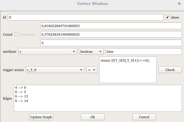 |
Vertex State Window |
| id |
the id of the vertex |
| coordinates |
the coordinates of the vertex. Note that the coordinates of ports are automatically computed |
| attribute |
Name type and value of the selected attribute. The definition of the attributes are done in the state window |
| Trigger action |
this box can be filled in only if the vertex is in the rule graph window. It specifies the new value of the selected attribute once the graph is rewritten. |
| Edges |
the list of the edges connected to the vertex |
| Update the graph |
apply the modifications to the vertex in the graph and see the result on the graph window |
| Ok |
apply the modifications to the vertex in the graph, see the result on graph window and close the window |
| Cancel |
cancel the modifications |
Edge state settings
To set the state of the edge, put the mouse's pointer on the edge and
click on the right button of the mouse. The edge popup menu appears. Select edit edge.
The following window appears:
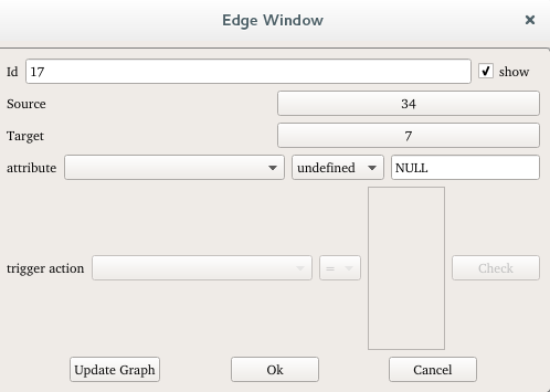 |
Edge State Window |
| id |
The id of the edge. |
| source |
the source vertex of the edge. A click on the button will make appear the corresponding vertex window |
| target |
the target vertex of the edge. A click on the button will make appear the corresponding vertex window |
| attribute |
name, type and value of the selected attribute. The definition of the attributes are done in the state window |
| Trigger action |
as for the vertex window, it specifies the new value of the selected attribute once the graph is rewritten. |
| Update the graph |
apply the modifications to the edge in the graph and see the result on graph window |
| Ok |
apply the modifications to the edge in the graph, see the result on graph window and close the window |
Cancel |
cancel the modifications |
Graph visualization and options
This section deals with the drawing options.
The result graphs can be very different depending on the initial graph and the rewriting system. Some graphs can have a large number of nodes. Some others can be not planar with a lot of crossing edges.
The presence of ports can complicate the readability of graphs. In some cases, only nodes are meaningful, in other cases, the visualization is better without the representation of ports and/or nodes.
To adapt the visualization to the current graph some options are available
in the second tool bar of the graph windows:
| Node |
by default the option is empty and the node is represented without labels. If id is chosen then all nodes are labeled by there corresponding id in the drawing. Whereas if one attribute is selected, then the state of each node will be represented by a color and a color scale appears at the right of the drawing. |
| Port |
by default the option is empty and the port is represented without labels. If id is chosen then all ports are labeled by there corresponding id in the drawing. Whereas if one attribute is selected, then the state of each port will be represented by a color and a color scale appears at the right of the drawing. |
| Edge |
by default the option is empty and the edge is represented without labels. If id is chosen then all edges are labeled by there corresponding id in the drawing. Whereas if one attribute is selected, then the state of each port will be represented by a color and a color scale appears at the right of the drawing. |
| Vertex size |
set the size of vertices |
| Edge width |
set the width of edges |
| show nodes |
by default the box is checked. If you do not want to visualize the nodes unchecked the box. |
| show ports |
by default the box is checked. If you do not want to visualize the ports unchecked the box. |
| show edges |
by default the box is checked. If you do not want to visualize the edges unchecked the box. |
To move on the drawing area:
- roll up the mouse 's wheel to zoom out or click on the
 button of the drawing area tools bar button of the drawing area tools bar
- roll down the mouse 's wheel to zoom in or click on the
 button of the drawing area tools bar button of the drawing area tools bar
- click on the left button of the mouse and by maintaining the left button pressed, select the drawing zone to fit
- click on the
 button of the drawing area tools bar to fit the best drawing zone which contains all the elements of the graph button of the drawing area tools bar to fit the best drawing zone which contains all the elements of the graph
- to move the drawing zone, click on the
 button of the drawing area tools bar and move the mouse. The drawing zone becomes read only. button of the drawing area tools bar and move the mouse. The drawing zone becomes read only.
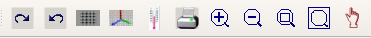 |
drawing area tools bar |
A graph window contains menu and corresponding tool bar.
|

|
Edit->Redo
|
Redo the last operation.
|
|

|
Edit->Undo
|
Undo the last operation.
|
|

|
Edit->Show grid
|
Show or mask the grid.
|
|

|
Edit ->Show Axes
|
Show or mask the axes.
|
|

|
Edit->Show Scales
|
Show or mask the scales.
|
|

|
Edit->Print
|
Print the graph on a printer.
|
|

|
Zoom - >Zoom +
|
Make a zoom centered in the graph window center.
|
|

|
Zoom -> Zoom -
|
Make the reverse operation of the preceeding operation.
|
|

|
Zoom-> Zoom Select
|
Select a zone of the graph to zoom in: select the rectangle
zone thanks to the mouse pointer.
|
|

|
Zoom -> Zoom Fit
|
Compute the zoom to fit the curves in the 2D Graph window.
|
|

|
Move->Move
|
Move the graph thanks to the mouse pointer. By pressing a
mouse click button, the graph will move like the mouse pointer and by
rolling the wheel, the graph may zoom in or zoom out.
|
To save the plotting area in a file
select File->save as image. The
image formats may be either bmp, png, ppm, xbm, xpm, jpg or .eps.
The
zoom may be selected precisely using the zoom setting window by
selecting Zoom->Zoom setting
|
|
|
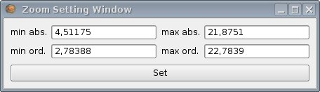
Zoom setting window
|
Set the min and
max absissa value and the min and max ordinate value and click set to
set the zoom rectangle exactly.
The options of the graph window
appear by selecting Edit->Options.
The different
options are listed below:
|
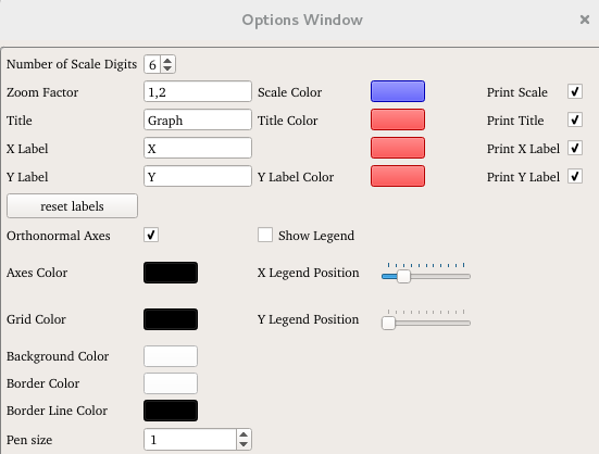
Number of scale digits
|
Number of scale digits on X and Y (rectangle 1).
|
|
Title
|
The name of the title (rectangle 2).
|
|
X Label
|
The name of the X Label (rectangle 3).
|
|
Y label
|
The name of the Y Label (rectangle 4).
|
|
Othonormal axes
|
The axes are normed.
|
|
Axes Color
|
The color of the axes.
|
|
Grid color
|
The color of the grid.
|
|
Background color
|
The color of the background.
|
|
Border Color
|
The color outside the border line.
|
|
Border line color
|
The color of the border line.
|
|
Scale color
|
The color of the X and Y scales.
|
|
Title color
|
The color of the title (rectangle 2).
|
|
X and Y label Color
|
The color of the X and Y label (rectangles 3 & 4).
|
|
Print Scale, Title, X label, Y Label
|
Print the scales, title, X or Y label or not.
|
show legend
|
Print the legend in the drawing
area.
|
|
X and Y legend position
|
The position of legend in plotting area (rectangle 5).
|
Pen size
|
Size of the pen for legends and
scales.
|
|